- Time to Read:
Most improvement projects and scientific research studies are conducted with sample data rather than with data from an entire population. A Probability Distribution is a way to shape the sample data to make predictions and draw conclusions about an entire population. It refers to the frequency at which some events or experiments occur. It helps finding all the possible values a random variable can take between the minimum and maximum statistically possible values.
Probability distributions are used to model real-life events for which the outcome is uncertain. Once we find the appropriate model, we can use it to make inferences and predictions. Line managers may use probability distributions to generate sample plans and predict process yields. Fund managers may use them to determine the possible returns a stock may earn in the future. Insurance managers may use them to forecast the uncertain future claims. Restaurant mangers may use them to resolve future customer complaints.
Probability runs on a scale of 0 to 1. If something could never happen, then it has a probability of 0. For example, it is impossible you could breathe and be under water at the same time without using a tube or mask. Conversely, if something is certain to happen, then it has a probability of 1. For example, it is certain that the sun will rise tomorrow.
You might be certain if you examine the whole population, but often times, you only have samples to work with. To draw conclusions from sample data, you should compare values obtained from the sample with the theoretical values obtained from the probability distribution. There will always be a risk of drawing false conclusions or making false predictions. Therefore, we need to be sufficiently confident before taking any decision by setting confidence levels (often set at 90 percent, 95 percent or 99 percent).
There are different shapes, models and classifications of probability distributions. They are often classified into two categories: discrete and continuous.
Discrete Probability Distributions
A Discrete Probability Distribution relates to discrete data. It is often used to model uncertain events where the possible values for the random variable are either attribute or countable. The two common discrete probability distributions are binomial and Poisson distributions.

The Binary Distribution (or Bernoulli distribution) is a discrete probability distribution that takes only two possible values. There is a probability that one value will occur and the other value will occur the rest of the time. Many real-life events can only have two possible outcomes, one of which can be considered as a success and the other as a failure. For example, a product can either pass or fail in an inspection test, a student can either pass or fail in an exam, and a tossed coin can either have a head or a tail.
The Binomial Distribution is a discrete probability distribution that is used for data which can only take one of two values (such as pass or fail, yes or no, or good or defective). It allows to compute the probability of the number of successes for a given number of trials or tests, each is either a success or a failure, given the probability of success on each trial. Success could mean anything you want to consider as a positive or negative outcome.
In Excel, you may calculate the binomial probabilities using the BINOM.DIST function. Simply write:
=BINOM.DIST(number of successes, number of trials, probability of success, FALSE)
Assume that you are tossing a coin 10 times, you will get a number of heads between 0 and 10. You may then carry out another 10 trials, in which you will also have a number of heads between 0 and 10. By doing this many times, you will have a data set which has the shape of the binomial distribution. In this case, getting a head would be a success (or a hit), the number of tosses would be the trials, and the probability of success is 50 percent.
The binomial test requires that each trial is independent from any other trial. In other words, the probability of the second trial is not affected by the first trial. This test has a wide range of applications, such as:
- Taking 10 samples from a large batch which is 3 percent defective (as past history shows).
- Asking the customers if they are going to shop again in the next 12 months.
- Counting the number of individuals who own more than one car.
- Counting the number of correct answers in a multiple-choice exam.
The Hypergeometric Distribution is very similar to the binomial distribution. The only difference is that a hypergeometric distribution does not use replacement between trials, and it is often used for samples from relatively small populations.
Assume that there are 5 gold coins and 25 silver coins in a box. You may close your eyes and draw 2 coins without replacement. By doing this many times, you will have a data set which has the shape of the hypergeometric distribution. You can then answer questions such as: what is the probability that you will draw one gold coin. Note that the probability of success on each trial is not the same as the size of the remaining population will change as you remove the coins.
It is not always appropriate to classify the outcome of a test simply as pass or fail. Sometimes, we have to count the number of defects where there may be several defects in a single item. The Poisson Distribution is a discrete probability distribution that specifies the probability of a certain number of occurrences over a specified interval (such as time or any other type of measurements).
In Excel, you may calculate the Poisson probabilities using the POISSON.DIST function. Simply write:
=POISSON.DIST(number of successes, expected mean, FALSE)
With the Poisson distribution, you may examine a unit of product, or collect data over a specified interval of time, in which you will have a number of successes (zero or more). You may then repeat the exercise, in which you will also have a number of successes. By doing this many times, you will have a data set which has the shape of the Poisson distribution. This test has a wide range of applications, such as:
- Counting the number of defects found in a single product.
- Counting the number of accidents per year in a factory.
- Counting the number of failures per month for a specific equipment.
- Counting the number of incoming calls per day to an emergency call center.
- Counting the number of customers who will walk into a store during the holidays.
Continuous Probability Distributions
A Continuous Probability Distribution relates to discrete data. It can take any value and can be measured with any degree of accuracy. The commonest and the most useful continuous distribution is the normal distribution. There are other continuous probability distributions that are used to model non-normal data such as: exponential, chi-square, etc.

The Uniform Distribution is a continuous probability distribution where the events have the exact same probability of happening anywhere within a fixed interval. It is often described as the rectangle distribution because it is typically looks like a rectangle. The mean is exactly halfway between the upper and the lower bounds. The uniform distribution does not occur often in nature, however, it is important as a reference distribution.
The Exponential Distribution is another continuous probability distribution that is often used in quality control and reliability analysis. It is mainly concerned with the amount of time until some specific event occurs. For example, we can use the exponential distribution to calculate the probability that a computer part will last less than six year. The shape of the exponential distribution is highly skewed to the right (there is a much greater area below the mean than above it).
The Normal Distribution is a symmetrical probability distribution where most results are located in the middle and few are spread on both sides. It has the shape of a bell and can entirely be described by its mean and standard deviation. Normality is an important assumption in many statistical tools and techniques when conducting statistical analysis so that they can be applied in the right manner.
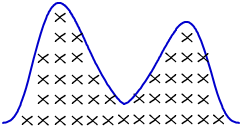
The Bimodal Distribution is a continuous probability distribution which has two modes (or peaks). In a bimodal distribution, two values occur more frequently than the other values. It can be seen, for example, in traffic analysis where traffic peaks during the morning rush hour and then again in the evening rush hour. A bimodal distribution may also result if the observations are taken from two different populations. This can be seen when taking samples from two different shifts or receiving materials from two different suppliers. In this case, there is actually one mode for the two data sets.

The bimodal is considered a Multimodal Distribution as it has more than one peak. This may indicate that your sample has several patterns of response, or has been taken from more than one population. Multimodal distributions can be seen in daily water distribution as water demand peaks during different periods of the day.


