- Time to Read:
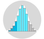
Continuous distributions describe variables that take values from a continuous range and can be measured with any degree of accuracy. The commonest and the most useful continuous distribution is the normal distribution. The Normal Distribution is a symmetrical probability distribution where most results are located in the middle and few are spread on both sides. It has the shape of a bell and can entirely be described by its mean and standard deviation.
The normal distribution can be found practically everywhere: in nature, in engineering and industrial processes, and in social and human sciences. Many everyday data sets follow approximately the normal distribution when compiled and graphed. For example, the body temperature for healthy humans typically follow the normal distribution. Other examples of normal data are the heights and weights of adults, the thickness and dimensions of a product, IQ and standardized test scores, and quality control test results.
In addition to being used to illustrate the shape and variability of the data, the normal distribution can be used to estimate future process performance. Normality is an important assumption in many statistical tools and techniques when conducting statistical analysis so that they can be applied in the right manner. Certain SPC charts, many process capability studies and many statistical inference tests require the data to be normally distributed.
The Normal Curve is a graphical representation of the normal distribution. It is determined by the mean and the standard deviation of the data. It a symmetric unimodal bell-shaped curve with its tails extending infinitely in both directions. The wider the curve, the larger the standard deviation and the more variation exists in the process. The spread of the curve is equivalent to six times the standard deviation of the process.
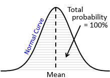
The normal curve helps calculating the probabilities for normally distributed populations. The probabilities are represented by the area under the normal curve where the total area under the curve is equal to 100 percent (or 1.00). By looking at the curve for any situation, we can get a rough estimate of the probability above a value, below a value, or between any two values. And since the normal curve is symmetrical, 50 percent of the data lie on each side of the curve.
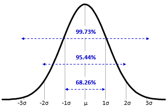
The normal distribution has a vary interesting and useful property regardless of the mean and standard deviation. For any normally distributed data, 68% of the data fall within one standard deviation of the mean, 95% of the data fall within two standard deviations of the mean, and 99.7% of the data fall within three standard deviations of the mean (nearly all of the data). This property is called the Empirical Rule or the 68–95–99.7 rule. Because of this property, you can quickly estimate the probability given the standard deviations from the mean.
Example
Suppose that the heights of a sample men are normally distributed with a mean height of 178 cm and a standard deviation of 7 cm. We can generalize that 68% of population are between 178 – 7 = 171 cm and 178 + 7 = 185 cm. This might be a generalization, but it’s true if the data is normally distributed.
Note: In Excel, you may calculate the normal probabilities using the NORM.DIST function. Simply write:
=NORM.DIST(x, mean, standard deviation, FALSE)
Where ‘x’ is the data point in question.
It is a common practice to convert any normal distribution to the standardized form and then use the standard normal table to find probabilities. The Standard Normal Distribution (Z distribution) is a way of standardizing the normal distribution. It always has a mean of zero and a standard deviation of one. Any normally distributed data can be converted to the standardized form using the formula: Z = (X – μ) / σ, where ‘X’ is the data point in question, and ‘Z’ (or Z-score) is a measure of the number of standard deviations of that data point from the mean. You can then use this information to determine the area under the normal distribution curve that is to the left of your data point, to the right of the data point, between two data points, or outside of two data points.
The complex shape of the normal curve has been converted into a mathematical table called the Z-table. The Z-table is used to find probabilities associated with the standard normal curve. You may also use the Z-table calculator instead of looking into the Z-table manually. There are different forms of the Z-table:
- Cumulative, which gives the proportion of the population that is to the left or below the Z-score.
- Complementary cumulative, which gives the proportion of the population that is to the right or above the Z-score.
- Cumulative from mean, which gives the proportion of the population to the left of that z-score to the mean only.
Example
Question: For a process with a mean of 100, a standard deviation of 10 and an upper specification of 120, what is the probability that a randomly selected item is defective (or beyond the upper specification limit)?
Answer:
In this case, the Z-score is equal to = (120 – 100) / 10 = 2. This means that the upper specification limit is 2 standard deviations above the mean.
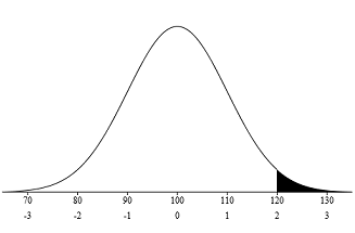
Now that we have the Z-score, we can use the Z-table to find the probability. From the Z-table (the complementary cumulative table), the area under the curve for a Z-value of 2 = 0.02275 or 2.275%. This means that there is a chance of 2.275% for any randomly selected item to be defective.
You may confirm your results by using this Z-Table Calculator.
Further Information
The normal distribution is also known as the Gaussian Distribution after Carl Gauss who created the mathematical formula of the curve.
Sometimes the process itself produces an approximately normal distribution. Other times the normal distribution can be obtained by performing a mathematical transformation on the data or by using means of subgroups.
The Central Limit Theorem is a useful statistical theory which states that the distribution of the means of random samples will always approach a normal distribution regardless of the shape and underlying distribution. Even if the population is skewed, the subgroup means will always be normal or near normal if the sample size is large enough. This theorem is a key concept because it implies that statistical methods that work for normal distributions can be applicable to other distributions. For example, certain SPC charts (such as XBar-R charts) can be used with non-normal data.
In Excel, you can generate random numbers that follow the normal distribution by using the NORM.INV function. Use the formula:
=NORM.INV(RAND(), mean, standard deviation).


