- Time to Read:
Descriptive statistics are methods of describing the characteristics of a data set. It includes calculating things such as the average of the data, its spread and the shape it produces. It involves describing, summarizing and organizing the data so it can be easily understood. Graphical displays are often used along with the quantitative measures to enable clarity of communication. Descriptive statistics helps exploring and making conclusions about the data in order to make more rational decisions.
Descriptive statistics are useful because they allow you to make sense of the data you are dealing with. For example, we may be concerned about measuring the weight of a product in a production line, or measuring the time taken to process an application. They aim to describe the data in a data set and help exploring the position, variability, shape and the outlier patterns of the data.
Before going any further, let’s define exactly what an outlier is. An Outlier is a data point that is significantly greater or smaller than other data points in a data set. It is useful when analyzing data to identify outliers because they may affect the calculation of descriptive statistics. Outliers can occur in any given data set and in any distribution. The easiest way to detect them is by graphing the data (i.e. using graphical methods such as histograms, box plots and normal probability plots).
In many cases, outliers may indicate an experimental error or incorrect recording of data (variability in the measurement). They may also occur by chance and it may be quite normal to have high or low data points. You need to think why they exist and decide whether to exclude them before carrying out your analysis. An outlier should be excluded if it is due to some type of error (i.e. measurement or human error), otherwise it should not.
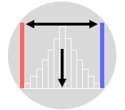
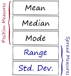
There are three measures that are used to describe a data set:
- Measures of position (also referred to as central tendency or location measures).
- Measures of spread (also referred to as variability or dispersion measures).
- Measures of shape.
Measures of Position
Position Statistics measure the data central tendency which refers to where the data is centered. You may have calculated an average of some kind. Despite the common use of average, there are different statistics by which we can describe the average of a data set.
The Mean of a data set is the total of all the data values divided by the size of the data set. It is the most commonly used statistic of position because it is easy to understand and calculate. It works well when the distribution is symmetric and there are no outliers. The mean of a sample is denoted by x-bar while the mean of a population is denoted by “μ”.
The Median of a data set is the middle value where exactly half of the data values are above it and half are below it. It is less widely used but a useful statistic due to its robustness. It can reduce the effect of outliers and often used when the data is nonsymmetrical. It is important to ensure that the values are ordered before calculating the median. Remember also that with an even number of values, the median is the mean of the two middle values.
The Mode is the value that occurs the most often in a data set. It is rarely used as a central tendency measure, it is more useful however to distinguish between unimodal and multimodal distributions (when data has more than one peak).
Measures of Spread
The Spread of the data refers to how the data deviates from the position measure (whether it is the mean or the median). It gives an indication of the amount of variation in the process which is an important indicator of quality. Remember that all manufacturing and transactional processes are variable to some degree, so it is important to have a measure of variability in order to control process variability and improve quality.
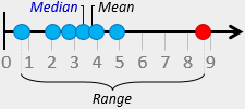
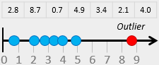
Median = 3.4 minutes
Range = 8.0 minutes
The Range of a data set is the difference between the highest and the lowest values. It is the simplest measure of variability and usually denoted by ‘R’. It is good enough in many practical cases, however, it does not make full use of the available data. It can be misleading when the data is skewed or in the presence of outliers. Just one outlier will increase the range dramatically.
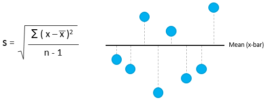
Standard Deviation is another measure of variability of the data. It is the average distance of the data points from their own mean. A low standard deviation indicates that the data points are clustered around the mean while a large standard deviation indicates that they are widely scattered around the mean. The standard deviation of a sample is denoted by ‘s’ while the standard deviation of a population is denoted by “μ”.
Standard deviation is perceived as difficult to understand because it is not easy to picture what it is. It is however a more robust measure of variability. Standard deviation is computed as follows:
Measures of Shape
Data can be plotted into a histogram to have a general idea of its shape, or distribution. The shape can reveal a lot of information about the data. Data will always follow some know distribution which may be symmetrical or nonsymmetrical. In a symmetrical distribution, the two sides of the distribution are a mirror image of each other. Examples of symmetrical distributions include: uniform, normal, camel-back, and bow-tie shaped.
The shape can also help identifying which descriptive statistic is more appropriate to use in a given situation. If the data is symmetrical for example, then it is appropriate to use the mean or median to measure the central tendency as they are almost equal. If the data is skewed, then the median will be a more appropriate to measure the central tendency.
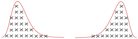
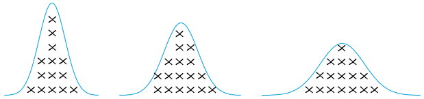
The two common statistics that measure the shape of the data are skewness and kurtosis. Skewness describes whether the data points are distributed symmetrically around the mean. A skewness value of zero indicates perfect symmetry. A negative value implies left-skewed data while a positive value implies right-skewed data. Skewness can be evaluated visually via a histogram and can be calculated by hand. But this is generally unnecessary with modern statistical software (such as Minitab).